Chapter 5 Combine, Reshape and Merge
This chapter looks at various strategies for combining, reshaping, and merging data.
5.1 Combine rows
Combining rows can be thought of as “stacking” rectangular data structures.
Python
The pandas function concat() binds rows together. It takes a list of pandas DataFrame objects. The second argument, axis, specifies a row bind when set to 0 and a column bind when set to 1. The default value is 0. The column names of the DataFrames should match; otherwise, the DataFrame fills with NaNs. You can bind rows with different column types.
import pandas as pd

d1 = pd.DataFrame({'x':[4, 5, 6], 'y':['a', 'b', 'c']})
d2 = pd.DataFrame({'x':[3, 2, 1], 'y':['d', 'e', 'f']})

# Create list of DataFrame objects
frames = [d1, d2]
combined_df = pd.concat(frames)

combined_df
x y
0 4 a
1 5 b
2 6 c
0 3 d
1 2 e
2 1 fThe following code is an example of when column names do not match, resulting in NaNs in the DataFrame.
# DataFrame with different column names
d1 = pd.DataFrame({'x':[4,5,6], 'z':['a','b','c']})
d2 = pd.DataFrame({'x':[3,2,1], 'y':['d','e','f']})

# Create list of DataFrame objects
frames = [d1, d2]
combined_df = pd.concat(frames)

combined_df
x z y
0 4 a NaN
1 5 b NaN
2 6 c NaN
0 3 NaN d
1 2 NaN e
2 1 NaN fR
As its name suggets, the rbind() function binds rows. It takes two or more objects as arguments. To row bind data frames, the column names must match, otherwise an error is returned. If the columns being stacked in the row bind have differing variable types, the values will be coerced according to the followig hierarchy: logical < integer < double < complex < character. (E.g., if you stack a set of rows with type logical in column J on a set of rows with type character in column J, the output will have column J as type character.)
d1 <- data.frame(x = 4:6, y = letters[1:3])
d2 <- data.frame(x = 3:1, y = letters[4:6])
rbind(d1, d2)
x y
1 4 a
2 5 b
3 6 c
4 3 d
5 2 e
6 1 fSee also the bind_rows() function in the dplyr package.
5.2 Combine columns
Combining columns can be thought of as setting rectangular data structures next to each other.
Python
The concat() function can be used to bind columns. Whereas we set axis to 0 above in order to bind rows, we set axis to 1 in order to bind columns. To column bind data frames, the number of rows must match; otherwise, the function throws an error.
d1 = pd.DataFrame({'x':[4, 5, 6], 'y':['a', 'b', 'c']})
d2 = pd.DataFrame({'z':[3, 2, 1], 'a':['d', 'e', 'f']})

# Create list of DataFrame objects
frames = [d1, d2]
combined_df = pd.concat(frames, axis=1)

combined_df
x y z a
0 4 a 3 d
1 5 b 2 e
2 6 c 1 fR
The cbind() function binds columns. It takes two or more objects as arguments. To column bind data frames, the number of rows must match; otherwise, the object with fewer rows will have rows “recycled” (if possible) or an error will be returned.
   x y  x
1 10 a 23
2 11 b 34
3 12 c 45
4 13 d 44
# Example of recycled rows (d1 is repeated twice)
d1 <- data.frame(x = 10:13, y = letters[1:4])
d2 <- data.frame(x = c(23, 34, 45, 44, 99, 99, 99, 99))
cbind(d1, d2) x y x
1 10 a 23
2 11 b 34
3 12 c 45
4 13 d 44
5 10 a 99
6 11 b 99
7 12 c 99
8 13 d 99See also the bind_cols() function in the dplyr package.
5.3 Reshaping data
The next two sections discuss how to reshape data from wide to long and from long to wide. “Wide” data are structured such that multiple values associated with a given unit (e.g., a person, a cell culture, etc.) are placed in the same row:
   name time_1_score time_2_score
1 larry            3            0
2   moe            6            3
3 curly            2            1
Long data, conversely, are structured such that all values are contained in one column, with another column identifying what value is given in any particular row (“time 1,” “time 2,” etc.):
     id time score
1 larry    1     3
2 larry    2     0
3   moe    1     6
4   moe    2     3
5 curly    1     2
6 curly    2     1
Shifting between these two data formats is often necessary for implementing certain statistical techniques or representing data with particular visualizations.
5.3.1 Wide to long
Python
To reshape a DataFrame from wide to long, we can use the pandas melt() function.
Consider the wide DataFrame below:
import numpy as np
import pandas as pd

data = {"id": [1, 2, 3],
        "wk1": np.random.choice(range(20), 3),
        "wk2": np.random.choice(range(20), 3),
        "wk3": np.random.choice(range(20), 3)}

df_wide = pd.DataFrame(data)
print(df_wide)
id wk1 wk2 wk3
0 1 2 19 0
1 2 6 10 17
2 3 17 1 15To take the DataFrame from wide to long with melt(), we specify the column(s) that uniquely identifies each row (id_vars), the variables containing the values to be lengthened (value_vars), and the name of the to-be-created column containing the lengthened values (value_name).
dataL = pd.melt(df_wide,
                # Column(s) that uniquely identifies/y each row
                id_vars = ["id"],
                # Variables that contain the values to be lengthened
                value_vars = ["wk1", "wk2", "wk3"],
                # Desired name of column in long data that will contain values
                value_name = "observations")
print(dataL)
id variable observations
0 1 wk1 2
1 2 wk1 6
2 3 wk1 17
3 1 wk2 19
4 2 wk2 10
5 3 wk2 1
6 1 wk3 0
7 2 wk3 17
8 3 wk3 15R
In base R, the reshape() function can take data from wide to long or long to wide. The tidyverse also provides reshaping functions: pivot_longer() and pivot_wider(). The tidyverse functions have a degree of intuitiveness and usability that may make them the go-to reshaping tools for many R users. We give examples below using both base R and tidyverse.
Say we begin with a wide data frame, df_wide, that looks like this:
  id sex wk1 wk2 wk3
1  1   m  16   7  15
2  2   m  12  19  10
3  3   f   8  15   7
To lengthen a data frame using reshape(), a user provides arguments specifying the columns that identify values’ origins (person, cell culture, etc.), the columns containing values to be lengthened, and the desired names for new columns in long data:
df_long <- reshape(df_wide,
                   direction = 'long',
                   # Column(s) that uniquely identifies/y each row
                   idvar = c('id', 'sex'),
                   # Variables that contain the values to be lengthened
                   varying = c('wk1', 'wk2', 'wk3'),
                   # Desired name of column in long data that will contain values
                   v.names = 'val',
                   # Desired name of column in long data that will identify each value's context
                   timevar = 'week')
df_long
id sex week val
1.m.1 1 m 1 16
2.m.1 2 m 1 12
3.f.1 3 f 1 8
1.m.2 1 m 2 7
2.m.2 2 m 2 19
3.f.2 3 f 2 15
1.m.3 1 m 3 15
2.m.3 2 m 3 10
3.f.3 3 f 3 7The tidyverse function for taking data from wide to long is pivot_longer() (technically housed in the tidyr package). To lengthen df_wide using pivot_longer(), a user would write:
library(tidyverse)
df_long_PL <- pivot_longer(df_wide,
# Columns that contain the values to be lengthened (can use -c() to negate variables)
cols = -c('id', 'sex'),
# Desired name of column in long data that will identify each value's context
names_to = 'week',
# Desired name of column in long data that will contain values
values_to = 'val')
df_long_PL# A tibble: 9 × 4
id sex week val
<int> <chr> <chr> <int>
1 1 m wk1 16
2 1 m wk2 7
3 1 m wk3 15
4 2 m wk1 12
5 2 m wk2 19
6 2 m wk3 10
7 3 f wk1 8
8 3 f wk2 15
9 3 f wk3 7pivot_longer() is particularly useful (a) when dealing with wide data that contain multiple sets of repeated measures in each row that need to be lengthened separately (e.g., two monthly height measurements and two monthly weight measurements for each person) and (b) when column names and/or column values in the long data need to be extracted from column names of the wide data using regular expressions.
For example, say we begin with a wide data frame, animals_wide, in which every row contains two values for each of two different measures:
animal lives_in_water jan_playfulness feb_playfulness jan_excitement
1 dolphin TRUE 6.0 5.5 7.0
2 porcupine FALSE 3.5 4.5 3.5
3 capybara FALSE 4.0 5.0 4.0
feb_excitement
1 7.0
2 3.5
3 4.0pivot_longer() can be used to convert this data frame to a long format where there is one column for each of the measures, playfulness and excitement:
animals_long_1 <- pivot_longer(animals_wide,
cols = -c('animal', 'lives_in_water'),
# ".value" is placeholder for strings that will be extracted from wide column names
names_to = c('month', '.value'),
# Specify structure of wide column names from which long column names will be extracted using regex
names_pattern = '(.+)_(.+)')
animals_long_1# A tibble: 6 × 5
animal lives_in_water month playfulness excitement
<chr> <lgl> <chr> <dbl> <dbl>
1 dolphin TRUE jan 6 7
2 dolphin TRUE feb 5.5 7
3 porcupine FALSE jan 3.5 3.5
4 porcupine FALSE feb 4.5 3.5
5 capybara FALSE jan 4 4
6 capybara FALSE feb 5 4 Alternatively, pivot_longer() can be used to convert this data frame to a long format where there is one column containing all the playfulness and excitement values:
animals_long_2 <- pivot_longer(animals_wide,
cols = -c('animal', 'lives_in_water'),
names_to = c('month', 'measure'),
names_pattern = '(.+)_(.+)',
values_to = 'val')
animals_long_2# A tibble: 12 × 5
animal lives_in_water month measure val
<chr> <lgl> <chr> <chr> <dbl>
1 dolphin TRUE jan playfulness 6
2 dolphin TRUE feb playfulness 5.5
3 dolphin TRUE jan excitement 7
4 dolphin TRUE feb excitement 7
5 porcupine FALSE jan playfulness 3.5
6 porcupine FALSE feb playfulness 4.5
7 porcupine FALSE jan excitement 3.5
8 porcupine FALSE feb excitement 3.5
9 capybara FALSE jan playfulness 4
10 capybara FALSE feb playfulness 5
11 capybara FALSE jan excitement 4
12 capybara FALSE feb excitement 4 5.3.2 Long to wide
Python
To reshape a DataFrame from long to wide, we can use the pandas pivot_table() function.
Consider the following long DataFrame:
import numpy as np
import pandas as pd
data = {"id": np.concatenate([([i]*3) for i in [1, 2 ,3]], axis=0),
"week": [1, 2, 3] * 3,
"observations": np.random.choice(range(20), 9)}
df_long = pd.DataFrame(data)
print(df_long) id week observations
0 1 1 9
1 1 2 0
2 1 3 14
3 2 1 0
4 2 2 15
5 2 3 19
6 3 1 14
7 3 2 4
8 3 3 0We can use pivot_table() to take the DataFrame from long to wide by specifying: the variable(s) that indicates each value’s source (index), the variable that indicates the context of each value (columns; e.g., “week 1,” “week 2,” etc.), and the variable containing the values to be widened (values).
df_wide = pd.pivot_table(df_long,
index = 'id',
columns = 'week',
values = 'observations')
print(df_wide)week 1 2 3
id
1 9 0 14
2 0 15 19
3 14 4 0R
Say that we begin with a long data frame, df_long, that looks like this:
      id sex week val
1.m.1  1   m    1  16
2.m.1  2   m    1  12
3.f.1  3   f    1   8
1.m.2  1   m    2   7
2.m.2  2   m    2  19
3.f.2  3   f    2  15
1.m.3  1   m    3  15
2.m.3  2   m    3  10
3.f.3 3 f 3 7To take the data from long to wide with base R’s reshape() function, a user would write:
df_wide <- reshape(df_long,
direction = 'wide',
# Column(s) that determine which rows should be grouped together in the wide data
idvar = c('id', 'sex'),
# Column containing values to widen
v.names = 'val',
# Column from which resulting wide column names are pulled
timevar = 'week',
# The `sep` argument allows a user to specify how the contents of `timevar` should be joined with the name of the `v.names` variable to form wide column names
sep = '_')
df_wide id sex val_1 val_2 val_3
1.m.1 1 m 16 7 15
2.m.1 2 m 12 19 10
3.f.1 3 f 8 15 7The tidyverse function for taking data from long to wide is pivot_wider(). To widen df_long using pivot_longer(), a user would write:
library(tidyverse)
df_wide_PW <- pivot_wider(df_long,
id_cols = c('id', 'sex'),
values_from = 'val',
names_from = 'week',
names_prefix = 'week_') # `names_prefix` specifies a string to paste in front of the contents of 'week' in the resulting wide column names
df_wide_PW# A tibble: 3 × 5
id sex week_1 week_2 week_3
<int> <chr> <int> <int> <int>
1 1 m 16 7 15
2 2 m 12 19 10
3 3 f 8 15 7pivot_wider() provides a great deal of functonality when widening relatively complicated long data structures. For example, say we want to widen both of the long versions of the “animals” data frame created above.
To widen the version of the long data that has a column for each of the measures (playfulness and excitement):
# A tibble: 6 × 5
  animal    lives_in_water month playfulness excitement
  <chr>     <lgl>          <chr>       <dbl>      <dbl>
1 dolphin   TRUE           jan           6          7
2 dolphin   TRUE           feb           5.5        7
3 porcupine FALSE          jan           3.5        3.5
4 porcupine FALSE          feb           4.5        3.5
5 capybara  FALSE          jan           4          4
6 capybara FALSE feb 5 4 animals_wide <- pivot_wider(animals_long_1,
id_cols = c('animal',
'lives_in_water'),
values_from = c('playfulness',
'excitement'),
names_from = 'month',
names_glue = '{month}_{.value}') # `names_glue` allows for customization of column names using "glue"; see https://glue.tidyverse.org/
animals_wide# A tibble: 3 × 6
animal lives_in_water jan_playfulness feb_playfulness jan_excitement
<chr> <lgl> <dbl> <dbl> <dbl>
1 dolphin TRUE 6 5.5 7
2 porcupine FALSE 3.5 4.5 3.5
3 capybara FALSE 4 5 4
# ℹ 1 more variable: feb_excitement <dbl>To widen the version of the long data that has one column containing all the values of playfulness and excitement together:
# A tibble: 12 × 5
   animal    lives_in_water month measure       val
   <chr>     <lgl>          <chr> <chr>       <dbl>
 1 dolphin   TRUE           jan   playfulness   6
 2 dolphin   TRUE           feb   playfulness   5.5
 3 dolphin   TRUE           jan   excitement    7
 4 dolphin   TRUE           feb   excitement    7
 5 porcupine FALSE          jan   playfulness   3.5
 6 porcupine FALSE          feb   playfulness   4.5
 7 porcupine FALSE          jan   excitement    3.5
 8 porcupine FALSE          feb   excitement    3.5
 9 capybara  FALSE          jan   playfulness   4
10 capybara  FALSE          feb   playfulness   5
11 capybara  FALSE          jan   excitement    4
12 capybara FALSE feb excitement 4 animals_wide <- pivot_wider(animals_long_2,
id_cols = c('animal', 'lives_in_water'),
values_from = 'val',
names_from = c('month', 'measure'),
names_sep = '_')
animals_wide# A tibble: 3 × 6
animal lives_in_water jan_playfulness feb_playfulness jan_excitement
<chr> <lgl> <dbl> <dbl> <dbl>
1 dolphin TRUE 6 5.5 7
2 porcupine FALSE 3.5 4.5 3.5
3 capybara FALSE 4 5 4
# ℹ 1 more variable: feb_excitement <dbl>5.4 Merge/Join
The merge/join examples below all make use of the following sample data frames:
  merge_var val_x
1         a    12
2         b    94
3 c 92 merge_var val_y
1 c 78
2 d 32
3 e 305.4.1 Left Join
A left join of x and y keeps all rows of x and merges rows of y into x where possible based on the merge criterion:

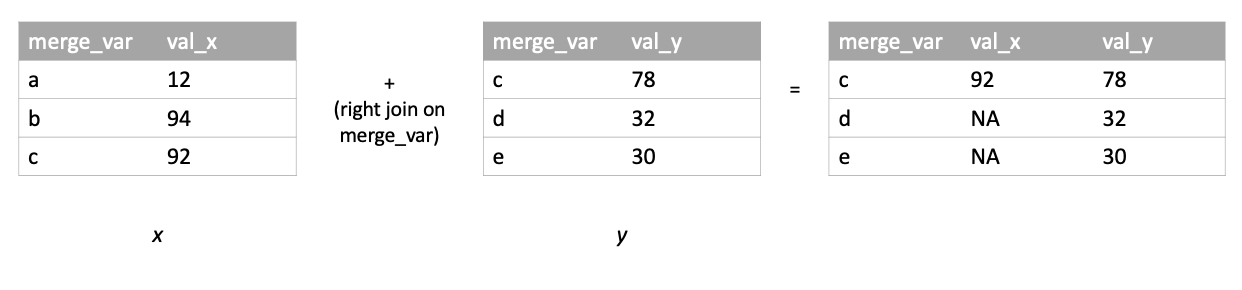
5.4.2 Right Join
A right join of x and y keeps all rows of y and merges rows of x into y wherever possible based on the merge criterion:
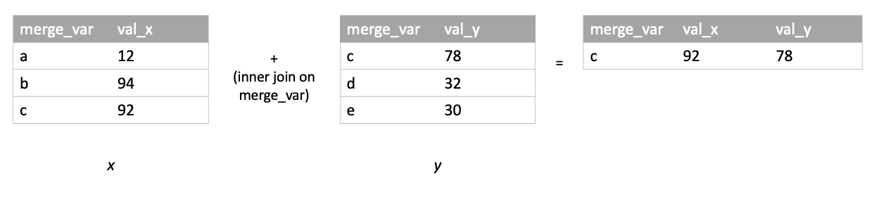
5.4.3 Inner Join
An inner join of x and y returns merged rows for which a match can be found on the merge criterion in both tables: