Generalized Additive Models
Generalized Additive Model with two predictors
Here, we will explore Generalized Additive Models (GAMs) in R using the {mgcv} package (Wood 2017). We will generate data for a baker who is passionate about sharing her love for baking and starts posting videos on a YouTube account. One of her first ‘how-to’ videos goes viral and she quickly gains over 50,000 subscribers!
To start, we will load our packages using library(). If
you do not have one or more of these packages, you can use the function
install.packages().
library(mgcv) # For fitting GAMs
library(ggplot2) #For plots
library(gratia) # For GAM validation
library(ggeffects) # For plotting model predictions
Let’s generate our data and take a look at the columns. In our data
frame, we will include the number of YouTube subscribers
(subscribers), number of video postings
(posts), and the length of the video in minutes
(vid.length).
#Reproducibility
set.seed(15)

#Generate a dataframe
df <- data.frame(subscribers =
                 pmax(50000 * (1 - exp(-0.1 * seq(0, 150, length.out = 150)))
                  + rnorm(150, mean = 0, sd = 2000), 0),
                 posts = seq(0, 150, length.out = 150),
                 vid.length = pmax(rnorm(150, mean = 8, sd = 3), 0))

#Examine the first 6 rows of data
head(df)
subscribers posts vid.length
1 517.6457 0.000000 7.366206
2 8450.7240 1.006711 6.442278
3 8439.1367 2.013423 8.921410
4 14827.9893 3.020134 9.907846
5 17549.8854 4.026846 1.699380
6 17264.2917 5.033557 7.572589Let’s go ahead and plot the data using the {ggplot2} package (Wickham 2016) to get an idea of the relationship between the number of subscribers and posts, which we will focus on throughout this tutorial.
ggplot(df, aes(x = posts, y = subscribers)) +
  geom_point() +
  labs(x = "Posts", y = "Subscribers", title = "Youtube Subscriber Growth") +
  theme_minimal()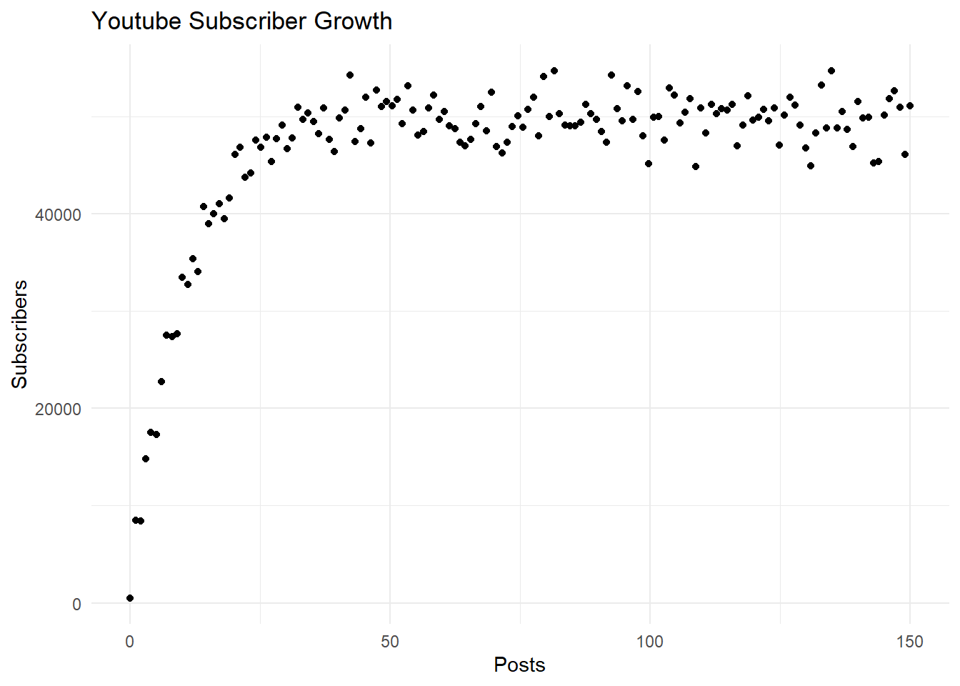
Let’s first try fitting a linear model to the data and then check the summary to see the results. The number of subscribers to YouTube will be predicted by the number of posts and video length.
#Fit a linear model
lm <- lm(subscribers ~ posts + vid.length, data = df)

#Check the linear model summary
summary(lm)
Call:
lm(formula = subscribers ~ posts + vid.length, data = df)

Residuals:
   Min     1Q Median     3Q    Max
-37241  -2768    913   4581  13646

Coefficients:
            Estimate Std. Error t value Pr(>|t|)
(Intercept)  33920.7     1994.1  17.010  < 2e-16 ***
posts          114.5       13.9   8.234 9.01e-14 ***
vid.length     521.1      197.4   2.640  0.00918 **
---
Signif. codes:  0 '***' 0.001 '**' 0.01 '*' 0.05 '.' 0.1 ' ' 1

Residual standard error: 7411 on 147 degrees of freedom
Multiple R-squared:  0.3311,    Adjusted R-squared:  0.322
F-statistic: 36.38 on 2 and 147 DF,  p-value: 1.457e-13
We can see that the predictor posts is significant. We
will evaluate model performance by looking at the plot of residuals
against the fitted values.
plot(lm, which = 1)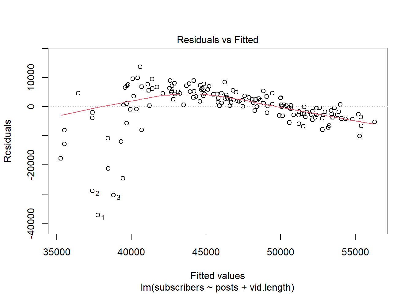
We see that this model does not perform very well with our data. The residuals have a clear pattern, highlighting that our model may not be capturing the structure of the data. Since the residuals display a non-linear pattern, we will fit a GAM to better capture the non-linearity.
We will use the gam() function in the {mgcv} package to
fit a GAM and add s() around our predictors to specify a
smoothing term for them. We are going to specify the argument
k = 9 to tell {mgcv} how ’wiggly` we think the smooth
should be, or how many basis functions can be used. The default value of
k is 10 for these smooths.
We will look at the summary to check the model output.
#Fit a GAM
gam1 <- gam(subscribers ~ s(posts, k = 9) + s(vid.length),
            method = "REML", data = df)

#Check the summary of our GAM model
summary(gam1)
Family: gaussian
Link function: identity

Formula:
subscribers ~ s(posts, k = 9) + s(vid.length)

Parametric coefficients:
            Estimate Std. Error t value Pr(>|t|)
(Intercept)  46562.5      187.6   248.2   <2e-16 ***
---
Signif. codes:  0 '***' 0.001 '**' 0.01 '*' 0.05 '.' 0.1 ' ' 1

Approximate significance of smooth terms:
                edf Ref.df   F p-value
s(posts)      7.795  7.986 262  <2e-16 ***
s(vid.length) 1.002  1.004   0   0.999
---
Signif. codes:  0 '***' 0.001 '**' 0.01 '*' 0.05 '.' 0.1 ' ' 1

R-sq.(adj) =  0.935   Deviance explained = 93.9%
-REML = 1370.6  Scale est. = 5.2796e+06  n = 150
We can see that our smooth for posts is statistically
significant and the deviance explained is high (94%) showing we were
able to explain the variation in our data well.
Importantly, smooths in a GAM are created by combining smaller
functions called basis functions. In this way, a non-linear relationship
between our independent and dependent variable has many parameters that
collectively create the overall smoothed shape we get for each term we
have specified a smooth for. However, we need to make sure our smoothing
terms are flexible enough to model the data as the basis dimensions
define how ‘wiggly’ the smooth function can be. We will check if the
basis size of our smoothing terms (k) is sufficient. To do this, we will
use the function k.check() on our GAM.
k.check(gam1) k' edf k-index p-value
s(posts) 8 7.794714 0.8666983 0.0525
s(vid.length) 9 1.002067 1.0647945 0.7800Notably, we can see that for posts, our k’ and edf
values are close to each other. The p-value for this smooth is also low
and the k-index falls below 1. These signs (1. a low p-value; 2. k’ and
edf close in value to each other; 3. k-index below 1) indicate that our
basis dimension (k) may be too low, and our model may benefit from a
higher k value. We can increase the k value by doubling it and seeing if
our edf value increases.
We will refit the GAM, specify a higher k value and call
k.check() again.
#Specify a GAM where `posts` has a k value of 18
gam2 <- gam(subscribers ~ s(posts, k = 18) + s(vid.length),
            method = "REML", data = df)

#Check the basis size of our smoothing terms for `gam2`
k.check(gam2)
k' edf k-index p-value
s(posts) 17 13.291363 1.069912 0.7750
s(vid.length) 9 1.001513 1.114679 0.9175We can now see that for posts, our k’ and edf values are
farther apart, our p-value is higher, and our k-index value is
approximately 1.
Fittting linear models and terms in mgcv
We can also fit a linear model with gam() by leaving out
the smoothing function. We will give it a try for comparison.
#Fit a linear model using `gam()`
lm <- gam(subscribers ~ posts + vid.length, data = df)

#Check the summary of `gam.lm`
summary(lm)
Family: gaussian
Link function: identity

Formula:
subscribers ~ posts + vid.length

Parametric coefficients:
            Estimate Std. Error t value Pr(>|t|)
(Intercept)  33920.7     1994.1  17.010  < 2e-16 ***
posts          114.5       13.9   8.234 9.01e-14 ***
vid.length     521.1      197.4   2.640  0.00918 **
---
Signif. codes:  0 '***' 0.001 '**' 0.01 '*' 0.05 '.' 0.1 ' ' 1


R-sq.(adj) =  0.322   Deviance explained = 33.1%
GCV = 5.6049e+07  Scale est. = 5.4928e+07  n = 150
Or, we could add a smoothing term and a linear term in the model by
including s() only around the terms we would like to
specify a smooth for.
gam.lm <- gam(subscribers ~ s(posts) + vid.length,
              method = "REML", data = df)

summary(gam.lm)
Family: gaussian
Link function: identity

Formula:
subscribers ~ s(posts) + vid.length

Parametric coefficients:
            Estimate Std. Error t value Pr(>|t|)
(Intercept) 46097.29     510.64   90.27   <2e-16 ***
vid.length     59.74      61.60    0.97    0.334
---
Signif. codes:  0 '***' 0.001 '**' 0.01 '*' 0.05 '.' 0.1 ' ' 1

Approximate significance of smooth terms:
          edf Ref.df     F p-value
s(posts) 8.74   8.98 270.9  <2e-16 ***
---
Signif. codes:  0 '***' 0.001 '**' 0.01 '*' 0.05 '.' 0.1 ' ' 1

R-sq.(adj) =  0.943   Deviance explained = 94.7%
-REML = 1363.9  Scale est. = 4.5997e+06  n = 150
Visualization & validation
Let’s go back to our gam2 model. We will plot the
estimated smooths of gam2 using partial effect plots.
Partial effect plots help us visualize how an individual term in the
model contributes to the overall prediction. In other words, each term
in our model contributes some amount to the overall prediction and the
partial effect plot helps us understand how a single term is associated
with the response. These plots are on the linear predictor scale (see
?plot.gam). For gam2, which has a Gaussian
family, the linear predictor scale is the response scale (i.e. the link
is identity). This determines the y axis of the partial effect
plots.
We will get 2 partial effect plots because we have 2 smooth terms. We
will add the partial residuals to the plot by including the argument
residuals = TRUE. The partial residuals account for other
partial effects. The small, vertical lines along the x-axis represent a
rug plot, indicating the distribution of the term shown. Standard errors
are represented by the dashed lines on the plot which show the 95%
confidence interval.
plot.gam(gam2, pages = 1,
         residuals = TRUE, # add partial residuals
         se = TRUE, shade = TRUE # add and shade the standard error
) 
Here, we see the average effect of each term is 0 with values above 0 having a positive contribution and values below 0 having a negative contribution.
We can help make the plot more interpretable by using the argument
shift which shifts the plot by a constant value. In our
case, we will shift the scale by the model intercept which is:
coef(gam2)[1](Intercept)
46562.51 plot.gam(gam2, shift = coef(gam2)[1], pages = 1) 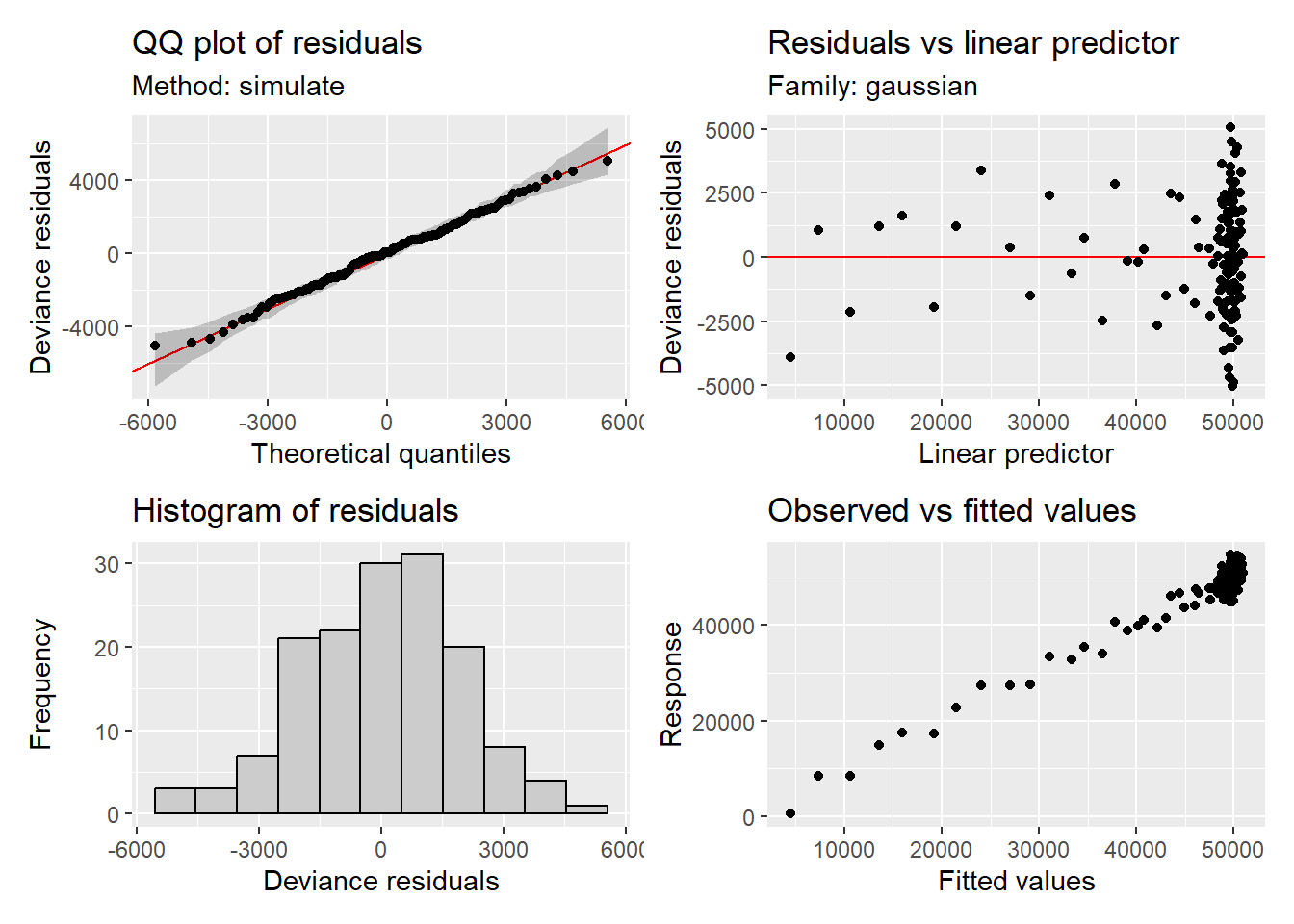
Notably, the shifted values should be interpreted with caution here as we have multiple smoothing terms.
We can also visualize the relationship between posts and subscribers
as predicted by the gam2 model using the package
{ggeffects} and include the raw data points.
predict.df <- ggpredict(gam2, terms = "posts")

ggplot() +
  #Raw data points
  geom_point(data = df, aes(x = posts, y = subscribers), color = "dodgerblue3", alpha = 0.5) +
  #Confidence intervals
  geom_ribbon(data = predict.df, aes(x = x, ymin = conf.low, ymax = conf.high), fill = "grey60", alpha = 0.5) +
  #Predicted values
  geom_line(data = predict.df, aes(x = x, y = predicted), color = "black", size = 1) +
  theme_classic()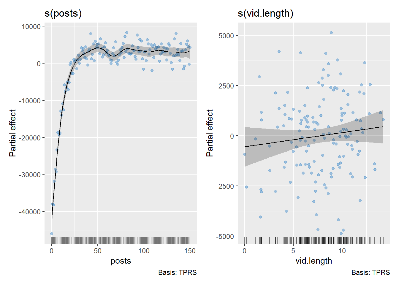
We can see the raw data points in blue, while the black line represents the model’s predicted values. The grey shaded area shows the confidence intervals around the predictions, giving us a sense of uncertainty in the model’s fit.
To further explore output on the response scale, see the {ggeffects} package.
Model diagnostics
To assess model diagnostics, we can also use gam.check()
from the mgcv package. The output from
gam.check() includes the information from
k.check() at the bottom of the results.
gam.check(gam2, pages = 1)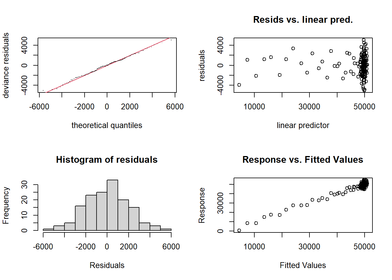
Method: REML   Optimizer: outer newton
full convergence after 7 iterations.
Gradient range [-0.0006043802,0.0001521058]
(score 1362.221 & scale 4366531).
Hessian positive definite, eigenvalue range [0.0006038669,74.04975].
Model rank =  27 / 27

Basis dimension (k) checking results. Low p-value (k-index<1) may
indicate that k is too low, especially if edf is close to k'.

                k'  edf k-index p-value
s(posts)      17.0 13.3    1.07    0.76
s(vid.length)  9.0  1.0    1.11    0.91
To assess model diagnostics, we can also use appraise()
from the {gratia} package (Simpson 2024).
Notably, this package is built on {ggplot2}, allowing for easy editing
of plots using ggplot scripts.
appraise(gam2, method = "simulate")
Within the {gratia} package, we can also plot the partial effect of
the smoothing terms. The smooths are centered around 0 so regions below
0 on the y-axis are less common on average while regions above 0 on the
y-axis are more common on average. We will add the residuals to the plot
by including residuals = TRUE.
draw(gam2, residuals = TRUE)
When specifying multiple smoothing terms, we can also check for
concurvity, which occurs when a smooth term in the model can be
estimated by one or more other smooth terms in the model. High
concurvity can lead to challenges with model interpretation. We can
check concurvity of our model using the {mgcv} function
concurvity(). The function will return values for 3 cases
ranging from 0 - 1 with 1 indicating high concurvity and potential
problems in the model. You can read more about how these cases are
calculated using ?concurvity.
concurvity(gam2) para s(posts) s(vid.length)
worst 2.591343e-22 0.32898939 0.3289894
observed 2.591343e-22 0.08288992 0.1881053
estimate 2.591343e-22 0.05899542 0.1728076While there is currently no defined value for what value is considered ‘high’ concurvity, our worst case estimate is 0.3 with the observed and estimated values falling below this. Here, we will conclude that concurvity is not a concern.